Sponsored Link

Sponsored Link

Monday, December 22, 2008

MS Excel, Macro & VBA e-books download

I wish to post all the E-books available on this earth on my blog. However, it is not practical to do so. I would request you to subscribe to blog via email to receive e-books and updates. As you subscribe, it becomes easier for me to send everyone at one go. I find the MS Excel help as the best help. Also, you can find lot of 'How to' on MS Excel Office web site.

http://office.microsoft.com/en-us/excel/FX100646961033.aspx

Kindly do let me know your comments about his post.

Read more on this article...

Tuesday, December 16, 2008

Understanding Visual Basic Editor in MS Excel

There are three main components that one should understand about Visual Basic Editor in MS Excel viz., Project Explorer, Properties and code window. All the version of MS Excel has same shortcut keys Alt + F11 key to bring up Visual Basic Editor in MS Excel. The picture shown below is Visual Basic Editor.

Click here to view enlarge

Microsoft Excel, VBE

Standard toolbar

Like any other Microsoft tool it comes along with ribbon toolbars. Shown below in the picture is standard toolbar which help you in performing various functions like run code, pause code and stop code which we will learn in details.

Click here to view enlarge

standard toolbar

Properties Window
Each object used in MS Excel has certain properties. These properties can be viewed in Properties window. We shall use these properties in examples ahead. In the picture below the properties window is showing the properties of sheet1. In case if you don’t find the properties window in VBE than press F4 key. F4 is shortcut key for bringing up Properties Window.

Properties are like the way you want the object to behave. Sometimes propertries are change on the runtime(While code is running). However, you can change all the properties at runtime

Click here to view enlarge

properties window

Project Explorer
Project Explorer shows all the Sheets, modules and classes presents in the project. Used of Project Explorer will be shown in the next post.

Click here to view enlarge

Microsoft Excel, Project Explorer

Code Window

Code windows is where you write your macro/VBA code. Code window has two drop downs one with the list of object as per the container selected in the project explorer. Like if Sheet1 is selected in the project explorer than you will find worksheet in left handside drop down. If the ThisWorkbook is selected then you will find Work in the left handside drop down. Similarly, you will find possible events listed in right handside drop down. For workbook you will find events like open, Window activate, Window deactivate etc. For worksheet, you will find events like SelectionChange etc

Click here to view enlarge

code window


Also, to add more to your knowledge about VBE. Visit following website : http://office.microsoft.com/en-us/help/HA010429591033.aspx

Feel free to comments about this post.  Also, you can receive free e-books, Add-ins, updates. Click here to Subscribe

We assure you knowledge, not SPAM!

Read more on this article...
Wednesday, December 10, 2008

VARIABLE Declaration in VBA

This will be shown only in post's page. Variable is used to store temporary information that is used for execution within the Procedure, Module or Workbook. Before we go into some detail of Variables, there are a few important rules that you must know about.

1) A Variable name must Start with a letter and not a number. Numbers can be included within the name, but not as the first character.
2) A Variable name cannot be longer than 250 characters.
3) A Variable name cannot be the same as any one of Excel's key words. By this, I mean you cannot name a Variable with such names as Sheet, Worksheet etc.
4) All Variables must consist of one continuous string of characters only. You can separate words by either capitalising the first letter of each word, or by using the underscore characters if you prefer.

You can name variables with any valid name you wish. For Example you could name a variable "Charles" and then declare it as any one of the data types shown below. However, it is good practice to formalize some sort of naming convention. This way when reading back your code you can tell at a glance what data type the variable is. An example of this could be the system I use! If you were to declare a variable as a Boolean (shown in table below) I may use: bIsOpen I might then use this Boolean variable to check if a Workbook is open or not. The "b" stands for Boolean and the "IsOpen" will remind me that I am checking if something is open.

You may see code that uses letters only as variables, this is bad programming and should be avoided. Trying to read code that has loads of single letters only can (and usually does) cause grief.

Mentioned below are the data types that can be used in VBA

Byte data type
A data type used to hold positive integer numbers ranging from 0 to 255. Byte variables are stored as single, unsigned 8-bit (1-byte) numbers. Useful when you know the maximum value that you want to store the in the variable.
Example below shows how to declare byte variable.

Dim btValue As Byte

Boolean data type
A data type with only two possible values, True (-1) or False (0). Boolean variables are stored as 16-bit (2-byte) numbers. Useful when you want to check certain value return after testing. Also, useful in controlling the program flow and you declare boolean its value is false by default

Dim blTest as boolean

Integer data type
Integer is most commonly used variable. A data type that holds integer variables stored as 2-byte whole numbers in the range -32,768 to 32,767. The Integer data type is also used to represent enumerated values. The percent sign (%) type-declaration character represents an Integer in Visual Basic.

Dim intCount As Integer

Long data type
A 4-byte integer ranging in value from -2,147,483,648 to 2,147,483,647. The ampersand (&) type-declaration character represents a Long in Visual Basic.

Dim lngCount As Long

Currency data type
A data type with a range of -922,337,203,685,477.5808 to 922,337,203,685,477.5807. Use this data type for calculations involving money and for fixed-point calculations where accuracy is particularly important. The at sign (@) type-declaration character represents Currency in Visual Basic.

Dim cur_profit As Currency

Single data type
A data type that stores single-precision floating-point variables as 32-bit (2-byte) floating-point numbers, ranging in value from -3.402823E38 to -1.401298E-45 for negative values, and 1.401298E-45 to 3.402823E38 for positive values. The exclamation point (!) type-declaration character represents a Single in Visual Basic.

Dim sngValue As Single

Double data type
A data type that holds double-precision floating-point numbers as 64-bit numbers in the range -1.79769313486232E308 to -4.94065645841247E-324 for negative values; 4.94065645841247E-324 to 1.79769313486232E308 for positive values. The number sign (#) type-declaration character represents the Double in Visual Basic.

Dim dbValue as Double

Date data type
A data type used to store dates and times as a real number. Date variables are stored as 64-bit (8-byte) numbers. The value to the left of the decimal represents a date, and the value to the right of the decimal represents a time.

Dim dtStart as date

String data type
A data type consisting of a sequence of contiguous characters that represent the characters themselves rather than their numeric values. A String can include letters, numbers, spaces, and punctuation. The String data type can store fixed-length strings ranging in length from 0 to approximately 63K characters and dynamic strings ranging in length from 0 to approximately 2 billion characters. The dollar sign ($) type-declaration character represents a String in Visual Basic.

Dim strName as String

Object data type
A data type that represents any Object reference. Object variables are stored as 32-bit (4-byte) addresses that refer to objects. Variant data type A special data type that can contain numeric, string, or date data as well as the special values Empty and Null. The Variant data type has a numeric storage size of 16 bytes and can contain data up to the range of a Decimal, or a character storage size of 22 bytes (plus string length), and can store any character text. The VarType function defines how the data in a Variant is treated. All variables become Variant data types if not explicitly declared as some other data type.

One small example of variable in macro is written below.

Sub VariableMacrotest()
Dim intEntervalue As Long
'Sheet1.Cells(1, 1) refers to A1 on sheet1
intEntervalue = Sheet1.Cells(1, 1)
MsgBox intEntervalue * intEntervalue
End Sub

To use the above code, press Alt + F11 to open the Visual Basic editor in MS Excel. If you don’t see the project explorer which by default on right hand side. Press Ctrl + R key. You will see the sheet MS Excel Worksheets. Right Click on the VBAProject(Workbookname) and go to insert and click on the module.
Copy past the code in the module and press F5 to run the macro/vba code.

Here I have attempted to put light on variable type available in MS Excel. I am sure this post was helpful. There are few more example I will post on variable in coming days.
 
Kindly subscribe to our blog via email to receive latest updates, its free.
 
We assure you knowledge, not SPAM!
Read more on this article...

Wednesday, December 3, 2008

Shortcut to move to Active Cell in Selection

This is the most common practice that I have observed in MS Excel user. If they select the large area on worksheet, they then use mouse to scroll and go back to active cells. The shortest way to go back to Active Cells is by pressing Ctrl Key + Backspace key

This post might not appear valuable to most of you readers. However, remember one thing. By using shortcuts you not only save your time. But exhibits how well you know the MS Excel to others users.

Also, do let me know your comments about this post and subscribe to us to receive latest updates via email

We assure you knowledge, not SPAM!

Read more on this article...

Prevent charts from being printed in MS Excel

Not all the time you want to print charts. Here is any trick prevent charts from being printed. Please follow the steps below. I am sure this will definitely help when you come across such scenario.

  • Select a chart, and right-click on chart. From the right click menu, select Format Chart Area.
  • Click on Properties tab, and remove the check from checkbox which says Print Object.
  • Click OK.

This trick is useful when you want to save your printer toner from preventing graph. If you like this post do let your comments and Subscribe via email

We assure you knowledge, not SPAM!

Read more on this article...

Tuesday, December 2, 2008

VBA advantages

The large portion of work in MS Excel can be achieved via macro and VBA. This post is an attempt to help MS Excel user with VBA. The post below provides an overview about Macro/VBA. In forth coming post I will tell you how to start VBA or in other words a VBA tutorial.

You can automate almost anything you do in Excel. To do so, you will have to write

Instructions that you want Excel to perform. Automating a task by using VBA offers several advantages:

Excel always executes the task in exactly the same way and with more consistency.

VBA performs the task much faster than you can do it manually.

If you’re a good macro programmer, Excel always performs the task without errors.

If you set things up properly, someone who doesn’t know anything about Excel can perform the task.

With MS Excel you can do things which are otherwise looks impossible — Also, it makes you popular in your work place

For long, time-consuming and monotonous tasks, Excel performs the entire task while you enjoy leisure

Under MS Excel help, VBA is little unexplored by most of the users. Everyone knows that’s things are possible using VBA. But, we look for work around. In next month, will post free tutorials based on VBA/Macro.

I hope you will like this post. Please express your view about this post via comments.

Also, you can subscribe to this post via email

We assure you knowledge, not SPAM!

Read more on this article...

Thursday, November 27, 2008

Accessing Outlook from MS Excel

The post will help you in exporting details like email id, sender's name, date and time of email lying in your Outlook inbox. Similarly, you can modify code to access to export/access other details from Outlook to MS Excel. If your now thinking what will be the use of this code. The answer is very simple, you can take the snapshot of your inbox and know what was the age of particular email at that point of time. Also, you can maintain list of emails from where you receive emails and at times you receive data or table in Outlook which you want to export in MS Excel.
Remember, we are here to provide free MS Excel help and enhance the MS Excel knowledge of all the blog visitors

Sub exportemail1()
'Code is free to use
'Do not remove comments
'for any further help, please visit
http://findsarfaraz.blogspot.com
‘for email me
findsarfaraz@gmail.com
On Error Resume Next
Dim emailcount As Integer
Dim OLF As Outlook.MAPIFolder
Dim ol As New Outlook.Application
'OLF is declared as mapi folder to decide'which folder you want to target
Set OLF = ol.Application.GetNamespace("MAPI").GetDefaultFolder(olFolderInbox)
'OLF.Items.Count provide the number of mail present in inbox
emailcount = OLF.Items.Count
'by i=1 we 'are initializing the variable by value 1'else it will throw an error
i = 1
'Here I am using do while - loop to'Browse through all mail
Do While i <= emailcount
Sheet3.Cells(i + 1, 1) = OLF.Items(i).SenderEmailAddress
Sheet3.Cells(i + 1, 2) = OLF.Items(i).SenderName
Sheet3.Cells(i + 1, 3) = OLF.Items(i).SentOn
i = i + 1
Loop
'Like SenderEmailAddress SenderName SentOn'we can use other properties of email to get other 'details
Set OLF = Nothing
Set ol = Nothing
End Sub

Though, this is only post so far. I will try my best to post more and more. Next, I am planning to post basic post on Vlookup, SUMIF and other basic function. For all these update you can subscribe via email.

Outlook to MS Excel Export Example download

We assure you knowledge, not SPAM!

Read more on this article...

Friday, October 24, 2008

Reverse the two words in MS Excel

Here we want to change Shivani Kumar to Kumar Shivani. It can be very useful when you want to change the data of First Name Last Name to Last Name First or vice versa.

Now lets take look at few basic ideas about develop

  1. Right(text, number of characters) function returns number of character of text starting from right. Example: Right(“Shivani Kumar”, 5) will return Kumar as a result
  2. Left(Text, number of characters) function returns number of characters of text starting from left. Example: Left(“Shivani Kumar”, 7) will return Shivani as a result
  3. Length on any text can be determine using LEN(text) function.Example : Len(“Shivani Kumar”) will return 13 as a result.
  4. Now the challenge is to find position of space in the text which can be done using Find(what to find, from where) function. Example : Find(“ “, “Shivani Kumar”) will return 8.

Now, we will combine the entire all the formulas to return reverse of two words.

MS Excel, reverse text trick

Formula: =RIGHT(A3,LEN(A3)-FIND(" ",A3))&" "&LEFT(A3,FIND(" ",A3)-1)

Here, we have learned and used three function viz LEFT(), RIGHT(), FIND(), LEN() which are basic. However, combining all together is an advance step.

We assure you knowledge, not SPAM!

Read more on this article...

Shortcuts to select Column(s) or Row(s)

I have impressed many in my team by using shortcuts in MS Excel and trust me this is an excellent trick. Also, you cannot remember all the shortcuts by reading them. The best way to learn shortcuts is learn one at a time and make sure that you bring that in practice.

Press Ctrl + Space key to select the entire column

Press Shift + Space key to select the entire row

Remember you can expand your selection by pressing shift key and arrows keys. A

After consciously trying few times, you will master this shortcut and whenever you need to select a column or row you will press Ctrl+Space and Shift + Space.

Subscribe via email, its free.

We assure you knowledge, not SPAM!

Read more on this article...

Wednesday, October 15, 2008

Find Day name in Excel

During this post we will try to find out methods to find Enclosed below are Four ways to find day name in Excel. Last one is easiest and very useful. During first way we will also attempt to write a VBA code which is a user define function.

1. Using VBA/User define function.


Public Function DayName(iDate As Date) As String
Day (iDate)

Select Case Weekday(iDate)
Case 1
DayName = "Sunday"
Case 2
DayName = "Monday"
Case 3
DayName = "Tuesday"
Case 4
DayName = "Wednesday"
Case 5
DayName = "Thursday"
Case 6
DayName = "Friday"
Case 7
DayName = "Saturday"
End Select

End Function

Enclosed at the bottom of post is example file with all three methods. To view code of user define function, press Alt + F11 key.

2. Using Lookup function.
Please look at the image below
lookupchoose
Formula : = LOOKUP(WEEKDAY(A2), {1,2,3,4,5,6,7},{"Sunday","Monday","Tuesday","Wednesday","Thursday","Friday","Saturday"})

2. Using Choose function.
Please look at the image below

 
daynamechoose


Formula : =CHOOSE(WEEKDAY(A2),"Sunday","Monday","Tuesday","Wednesday","Thursday","Friday","Saturday")
2. Using Text function.
Please look at the image below

daynametext

Formula: = Text(A2, "DDDD")

Note: this is one method suggested to me via comment. Hence I always appreciate comments. Also, you can subscribe via email.

Click here to download example

We assure you knowledge, not SPAM!


Read more on this article...

Sunday, October 12, 2008

Offset Function MS Excel

Offset Function and its uses

In the simple words, OFFSET function returns the value in cell which is certain number of rows and column aways from base(reference cell) cell. Also, it can provide you with range when used with other functions like sum, avg, etc.

Offset require the following parameter

  1. Reference:  Reference is place where you with to place your Offset Origin
  2. Row:  Row from where you start  the Offset
  3. Col : Column from where you start the Offset
  4. Height:  Height of the range (which will be an numeric)
  5. Weight : Weight of the range
  6. Now lets look at the following example which describe the Offset function.
  7. In the following example offset is starting at cell C2,
  8. Referece = C2
  9. Row= 1  which means next row to C2 ->C3
  10. Column =-1 which means the one column before C3 which is B3
  11. Since we are only using Offset  to return value we will provide height as 1.

Height parameter is useful when we want range to be returned as a reference.  Like when you want to provide dynamic range to SUM function or Data Validation.

Please download the example to see examples on dynamic range.

Offset Function

We would like to see your comments about this post. Also, you can receive email whenever we update. Just CLICK HERE 

We assure you knowledge, not SPAM!

Read more on this article...

Saturday, October 11, 2008

Contact Me

Please feel free to write to us your feedback. Also, write to us about topic in MS Excel that you like us to post on this blog.
Your Name
Your Email Address
Subject
Message
Image Verification
Please enter the text from the image
[ Refresh Image ] [ What's This? ]

Note: We will only reply to those email addresses which are subscribed to this blog. If you have not subscribed than Click here Read more on this article...

Wednesday, October 8, 2008

Now, Submit your MS Excel tips

Now here is chance to share your knowledge with other users across world. Also, along with your MS Excel tip you can leave link to your web site/blog. We appreciate your help.

Your Name
Your Email Address
Subject
File Attachment
Message
Image Verification
Please enter the text from the image
[ Refresh Image ] [ What's This? ]

Note: Please do not use this form to ask queries. Read more on this article...

Tuesday, October 7, 2008

Uses of Indirect Function in Excel

Here, we are trying to explore the help on INDIRECT function in MS Excel. The MS Excel help example listed below is free to download. Please use that as it will help in clarifying your doubts indirect function

  1. Indirect() basically needs the reference like A4
  2. Suppose if you try =Indirect(“A4”) in the cell B2 then it will return value present in A4
    Also, I have enclosed the excel with example with application of indirect formula. I am sure this example would help you in using this formula on the job scenario.

Click here to download Example

We assure you knowledge, not SPAM!

Read more on this article...

Shade alternate rows using conditional Formatting

This post is very useful when you want to make your reports look really professional without spending lot of time. There are many templates provided by Microsoft which has alternate shaded rows.

MS Office 2003:

1. Select all the row and columns using CTRL + A keys on keyboard or by clicking on top left hand side corner.
2. Click on Format Menu -> Select Condition Formatting.
3. From the drop down, select the option Formula.
4. Enter the Formula enter =MOD(ROW(),2)
5. Row() function returns the number of row 1, 2, 3 and so on and Mod function basically return you the remainder after the division by 2

  • Mod ( 1 ,2 ) will return 1
  • Mod(2,2) will return 0
  • Mod (3,2) will return 1

6. Click on format button
7. Select the patterns tab and select the suitable color
8. Click on Ok and Ok.

In the above example, we learned two functions ROW() and MOD(). In future, I will post more functions which will use these functions in combination with other functions.

Also, do post your comments about this post and CLICK HERE to see updates on your email.

Read more on this article...

Advertise with us

We got page rank 2 in  Google and we constantly work on content of our blog to provide user friendly help in MS Excel. We have around 4500 visits each month and 5500 page views. If you wish to advertise here, please select the section of page where you want to put your advertisement and proceed with payment. We advertise in 125 X 125 pixel square ads only. Also, we will put on your ads as soon as payment to my account and ad image is received in.  For any other offer, please feel free to write me.

Banner Type
Read more on this article...

Thursday, October 2, 2008

Privacy Policy for findsarfaraz.blogspot.com

If you require any more information or have any questions about our privacy policy, please feel free to contact us by email at findsarfaraz@gmail.com.
At findsarfaraz.blogspot.com, the privacy of our visitors is of extreme importance to us. This privacy policy document outlines the types of personal information is received and collected by findsarfaraz.blogspot.com and how it is used.
Log Files
Like many other Web sites, findsarfaraz.blogspot.com makes use of log files. The information inside the log files includes internet protocol ( IP ) addresses, type of browser, Internet Service Provider ( ISP ), date/time stamp, referring/exit pages, and number of clicks to analyze trends, administer the site, track user’s movement around the site, and gather demographic information. IP addresses, and other such information are not linked to any information that is personally identifiable.
Cookies and Web Beacons
findsarfaraz.blogspot.com does use cookies to store information about visitors preferences, record user-specific information on which pages the user access or visit, customize Web page content based on visitors browser type or other information that the visitor sends via their browser.
DoubleClick DART Cookie
.:: Google, as a third party vendor, uses cookies to serve ads on findsarfaraz.blogspot.com.
.:: Google's use of the DART cookie enables it to serve ads to users based on their visit to findsarfaraz.blogspot.com and other sites on the Internet.
.:: Users may opt out of the use of the DART cookie by visiting the Google ad and content network privacy policy at the following URL - http://www.google.com/privacy_ads.html
Some of our advertising partners may use cookies and web beacons on our site. Our advertising partners include ....
Google Adsense
These third-party ad servers or ad networks use technology to the advertisements and links that appear on findsarfaraz.blogspot.com send directly to your browsers. They automatically receive your IP address when this occurs. Other technologies ( such as cookies, JavaScript, or Web Beacons ) may also be used by the third-party ad networks to measure the effectiveness of their advertisements and / or to personalize the advertising content that you see.
findsarfaraz.blogspot.com has no access to or control over these cookies that are used by third-party advertisers.
You should consult the respective privacy policies of these third-party ad servers for more detailed information on their practices as well as for instructions about how to opt-out of certain practices. findsarfaraz.blogspot.com's privacy policy does not apply to, and we cannot control the activities of, such other advertisers or web sites.
If you wish to disable cookies, you may do so through your individual browser options. More detailed information about cookie management with specific web browsers can be found at the browsers' respective websites.

Read more on this article...

Tuesday, September 30, 2008

To remove empty rows between data

There are many ways to remove empty rows from table. One way I prefer is by moving all empty rows to bottom by using sort.
To remove empty rows between data:

1. Select all columns containing data by pressing Ctrl+Shift+End.
2. Click the Sort icon under Data menu(Office 2003 or below) (either Ascending or Descending).

As the purpose of this blog is to train/help all MS Excel users. You will find all the examples from basic to advance. Thanks for spending time in reading this post. Do leave valuable comments
 
Subscription is free here. Click here to subscribe
Read more on this article...

Find how many times a particular character repeats in a cell.

LEN function is used to find the total length of text and Substitute function is used to replace one letter with some other letter on all instance.  Like If the cell A1 contains text 'Safaraz Ahmed' and I want to find out how many times character 'a' is repeat in cell A1.
 
1. Type Sarfaraz Ahmed in cell A1
2. Type a in the cell A2.
Click on image below to view Enlarge
 
sub
 
3. Enter the following formula in A3: =  LEN(A1)-LEN(SUBSTITUTE(A1,A2,""))
SUBSTITUTE(A1, A2,"") will replace 'a' with '' from Sarfaraz ahmed to return Srfrz hmed
which is of length 10 as it also include space.
4. LEN(A1) returns the length text including 'a' which is 14.
5. LEN(A1)-LEN(SUBSTITUTE(A1,A2,""))  returns 4.
Kindly provide your valuable comments.
Read more on this article...

Friday, September 26, 2008

Find and replace ?

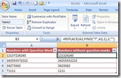
Find and replace is very common thing we can expect from any application. However, certain special character can't be replaced like question mark '?'. But this can be very well tricked by using Replace function.

1.  When you want use find & replace to remove ? from the string you will notice that all the next old text will be replaced by new text.

2.  The following formula will replace ?(question mark) from the string.

3.  Remember only one ? mark.

findreplace
Formula is mentioned below:
=REPLACE(A2,FIND("?",A2,1),1,"")
 
Subscribe via email to receive more trick right in your inbox.
 
We assure you knowledge, not SPAM!
Read more on this article...

Wednesday, September 24, 2008

Import data from website to MS Excel

Many times we don't want to go to website again and again to check if content is updated. Alternative is to import such data to MS Excel. This post will help you in understanding how to import data to MS Excel. Please carefully read the instruction below.

To import and refresh information from a Web site:

1. Open MS Excel XP/ 2003, and click on the Data menu, click Import External Data, and then New Web Query.
2. In the Address box of the New Web Query dialog box, type or paste the address of the Internet site which you want to see on your excel sheet

For example, open the site www.bloomberg.com, which includes a table of various currency exchange rates. The address of the page containing the table of currency exchange rates is http://www.bloomberg.com/markets/index.html.
3. In the dialog box, notice the Web page. Click the small arrow in the upper left-hand corner of the table to select only the data table.
4. Click Import.
5. To save the query, click Properties in the
Import Data dialog box.
6. In the External Data Range Properties dialog box, enter the query name in the Name box, select the Save Query definition checkbox, and then click OK.
7. In the Import Data dialog box, click OK to import.

To refresh the Internet data


1. Select the cell in the sheet containing the data.
2. From the Data menu, select Refresh Data.
OR
Display the External Data toolbar and click the Refresh Data icon. To display the External Data toolbar, select one of the toolbars, right-click and select External Data, and click OK
.

To automatically refresh the Internet data:

1. On the External Data toolbar, click the Data Range Properties icon.
2. Select the Refresh every option, and set the number of minutes between each refresh action.
3. Select the Refresh data on file open checkbox to automatically refresh the data when the file is opened.

Do let me know your comments and experience about using information provided in this post via comments. Also, subscribe via email to receive latest updates, add-ins and ebooks on MS Excel.

D

Read more on this article...

Monday, September 22, 2008

Check which CASE is used using Exact function

The formula is not very useful in practical MS Excel application. However, can be use to improve your knowledge about EXACT function.

Exact function basically compares the text from two cells for all aspects like content and case both. For Example, If cell A1 contains S and B1 contains s then the formula Exact (A1, B1) will return false.

Upper functions converts any case into Upper case.

Lower function converts any case into Lower case.

Proper function converts any case into Proper case (First letter of each word capital).

Formula:
=IF(EXACT(C9,UPPER(C9)),"UPPER CASE",IF(EXACT(C9,LOWER(C9)),"LOWER",(IF(EXACT(C9,PROPER(C9)),"PROPER","INCORRECT CASE"))))

In this trick,  IF Exact(C9, Upper(Exact(C9))  returns true only if C9 is in upper case and same goes other cases.

This formula may not be very useful in practical application. However, very useful in understanding Exact function.

Thank you for spending your valuable time in reading above post and if you like to read more such tricks subscribe to blog via email.

We assure you knowledge, not SPAM!

Read more on this article...

How to Remove Apostrophe

Suppose if column A contains an imported list of numbers. All these number will have an invisible apostrophe due to which MS Excel interprets such numbers as text. These numbers can’t be formatted as currency or they cannot be using in calculation as SUM and AVERAGE. From office XP onward you can recognize them by a triangular green color mark at the left side top of the cell.

We will have to convert them into values/numbers, so we can use them in formulas or format them as currency.

Please have a look at the steps below
Office XP or Above:
1. Select the enter column from which you wish to remove apostrophe. On the highlighted cell, you will see an exclamation mark .
2. Click on the exclamation mark and select Convert to Number from menu.

Office 2000:
You will have to use the VALUE function as shown in the following

Formula:

=VALUE(A1)

Subscribe here to receive more such tips. Your comments motivate us to post more.

We assure you knowledge, not SPAM!

Read more on this article...

Saturday, September 20, 2008

Calculate Six Sigma in Excel

Sigma is calculated using error and number of opportunities. At times, people need different tool for calculating Sigma. At times, people even search in Google. I wish if you reach here and understand Sigma calculation once an and all in MS Excel.

  1. The Six Sigma mainly consist defects/error and Total number of opportunities.
  2. Please check the formula in the image below. For reference use, it's mentioned below.

sixsigma

Formula:

=IF(A2=0,6,IF(A2=B2,0,IF(B2=0, "DENOMINATOR CANNOT BE ZERO",ROUND((NORMSINV(1-A2/B2)+1.5),2))))

If you like this post, spend two minutes in leaving comments. To receive update over email do subscribe to us.

We assure you knowledge, not SPAM!

Read more on this article...

Separate Text based on SPACE

This post describe a scenario where you have list of first name and last name separated by space and you want to take only first name. In other words you have two word separated by text and you want result as only first part as result.
 
The following formula will separate the text part based on the position of space in the text.
You can see the formula in formula bar of image. Also the same is mentioned below
Formula
=LEFT(A2,FIND(" ",A2,1))

MS Excel, Text Separate
 

Also, do let me know your comments about this post and subscribe to us to receive latest updates via email

We assure you knowledge, not SPAM!

Read more on this article...

Friday, September 19, 2008

User Define function to Convert Number to Text

This function is something I wrote myself on request of one of my community member from my MS Excel community on Orkut.  Through this post  I am also attempting to teach blog readers how to move code to Visual Basic Editor for use.

The Function will convert 122 into One Hundred and Twenty Two
1. Press ALT + F11 to start Vb Editor
2. Insert Module
3. Copy paste the entire code into module
4. Check the function in the list of User Define Function.
e.g = N2T(a2)
Where a2 cell contain numeric value

'The below program is written to convert the number into text
'The logic in solely developed by Sarfaraz Ahmed and is not referred from any internet on internet or any book
'Hence, user in this forum can freely use the function.
'User are requested not to remove the comments


Dim fplace(0 To 20) As String
Dim splace(0 To 10) As String
Dim PlaceName(1 To 5) As String
Private Sub LoadValue()

fplace(0) = ""
fplace(1) = "One"
fplace(2) = "Two"
fplace(3) = "Three"
fplace(4) = "Four"
fplace(5) = "Five"
fplace(6) = "Six"
fplace(7) = "Seven"
fplace(8) = "Eight"
fplace(9) = "Nine"
fplace(10) = "Ten"
fplace(11) = "Eleven"
fplace(12) = "Twelve"
fplace(13) = "Thirteen"
fplace(14) = "Fourteen"
fplace(15) = "Fifteen"
fplace(16) = "Sixteen"
fplace(17) = "Seventeen"
fplace(18) = "Eighteen"
fplace(19) = "Nineteen"
fplace(20) = "Twenty"


splace(0) = ""
splace(1) = "Ten"
splace(2) = "Twenty"
splace(3) = "Thirty"
splace(4) = "Forty"
splace(5) = "Fifty"
splace(6) = "Sixty"
splace(7) = "Seventy"
splace(8) = "Eight"
splace(9) = "Ninety"
splace(10) = "Hundredth"


PlaceName(1) = "Hundred"
PlaceName(2) = "Thousand"
PlaceName(3) = "Lakh"
PlaceName(4) = "Crore"
End Sub

Function N2T(DbVal As Double) As String
LoadValue
Dim LFTPART As String
Dim RGTPART As String
Dim RGTLEN As Integer
Dim LFTLEN As Integer


If Len(Trim(DbVal)) < 3 Then
N2T = D2T(DbVal)
ElseIf Len(Trim(DbVal)) = 3 Then
N2T = D2T(Left(DbVal, 1)) & " " & CheckZero(Left(DbVal, 1), "Hundred") & " " & CheckZero(Right(DbVal, 2), "And") & " " & D2T(Right(DbVal, 2))
ElseIf Len(Trim(DbVal)) = 4 Then
N2T = D2T(Left(DbVal, 1)) & " " & CheckZero(Left(DbVal, 1), "Thousand") & " " & D2T(Mid(DbVal, 2, 1)) & " " & CheckZero(Mid(DbVal, 2, 1), "Hundred") & " " & CheckZero(Right(DbVal, 2), "And") & " " & D2T(Right(DbVal, 2))
ElseIf Len(Trim(DbVal)) = 4 Then
N2T = D2T(Left(DbVal, 1)) & " " & CheckZero(Left(DbVal, 1), "Thousand") & " " & D2T(Mid(DbVal, 2, 1)) & " " & CheckZero(Mid(DbVal, 2, 1), "Hundred") & " " & CheckZero(Right(DbVal, 2), "And") & " " & D2T(Right(DbVal, 2))
ElseIf Len(Trim(DbVal)) = 5 Then
N2T = D2T(Left(DbVal, 2)) & " " & CheckZero(Left(DbVal, 1), "Thousand") & " " & D2T(Mid(DbVal, 3, 1)) & " " & CheckZero(Mid(DbVal, 3, 1), "Hundred") & " " & CheckZero(Right(DbVal, 2), "And") & " " & D2T(Right(DbVal, 2))
ElseIf Len(Trim(DbVal)) = 6 Then
N2T = D2T(Left(DbVal, 1)) & " " & CheckZero(Left(DbVal, 1), "Lakh") & " " & D2T(Mid(DbVal, 2, 2)) & " " & CheckZero(Mid(DbVal, 2, 2), "Thousand") & " " & D2T(Mid(DbVal, 4, 1)) & " " & CheckZero(Mid(DbVal, 4, 1), "Hundred") & " " & CheckZero(Right(DbVal, 2), "And") & " " & D2T(Right(DbVal, 2))
ElseIf Len(Trim(DbVal)) = 7 Then
N2T = D2T(Left(DbVal, 2)) & " " & CheckZero(Left(DbVal, 2), "Lakh") & " " & D2T(Mid(DbVal, 3, 2)) & " " & CheckZero(Mid(DbVal, 3, 2), "Thousand") & " " & D2T(Mid(DbVal, 5, 1)) & " " & CheckZero(Mid(DbVal, 5, 1), "Hundred") & " " & CheckZero(Right(DbVal, 2), "And") & " " & D2T(Right(DbVal, 2))
ElseIf Len(Trim(DbVal)) = 8 Then
N2T = D2T(Left(DbVal, 1)) & " " & CheckZero(Left(DbVal, 1), "Crore") & " " & D2T(Mid(DbVal, 2, 2)) & " " & CheckZero(Mid(DbVal, 2, 2), "Lakh") & " " & D2T(Mid(DbVal, 4, 2)) & " " & CheckZero(Mid(DbVal, 4, 2), "Thousand") & " " & D2T(Mid(DbVal, 6, 1)) & " " & CheckZero(Mid(DbVal, 6, 1), "Hundred") & " " & CheckZero(Right(DbVal, 2), "And") & " " & D2T(Right(DbVal, 2))
ElseIf Len(Trim(DbVal)) = 9 Then
N2T = D2T(Left(DbVal, 2)) & " " & CheckZero(Left(DbVal, 2), "Crore") & " " & D2T(Mid(DbVal, 3, 2)) & " " & CheckZero(Mid(DbVal, 3, 2), "Lakh") & " " & D2T(Mid(DbVal, 5, 2)) & " " & CheckZero(Mid(DbVal, 5, 2), "Thousand") & " " & D2T(Mid(DbVal, 7, 1)) & " " & CheckZero(Mid(DbVal, 7, 1), "Hundred") & " " & CheckZero(Right(DbVal, 2), "And") & " " & D2T(Right(DbVal, 2))
Else
N2T = "Value is too big, function support upto 9 digits only"
End If

End Function
Private Function D2T(intVal As Double) As String
If intVal > 20 Then
D2T = splace(Left(intVal, 1)) & " " & fplace(Right(intVal, 1))
Else
D2T = fplace(intVal)
End If
End Function


Private Function CheckZero(intVal As Double, PlaceName As String) As String
If intVal = 0 Then
CheckZero = ""
Else
CheckZero = PlaceName
End If

End Function

Read more on this article...