Sponsored Link

Sponsored Link

Wednesday, August 19, 2009

VBA code, extract Number from Text

During this post I will try to share VBA/Macro code to extract number from the text. Also, we will discuss the code to help you in understanding how to code in VBA. After all the aim is to make you enable write VBA code. Though in most of my post I write this at the end. This time I am advising you in middle to subscribe yourself to this blog. Also, your comments motivates us.

Let's move ahead with first understanding the application/scenario under which you can use this code. Take an example where you Microsoft Excel file where you have series of number where text is between number and you are only interested in numbers and not next. If the text is on fixed place you can remove that using LEFT() , RIGHT() or MIDDLE() function. But if the numbers and text are placed in cell where you are not sure number of text character and position of text. VBA code is solution to extract number.

VBA code to extract Number from Text

Function ExtractNumber(Target As Range) As Variant
Dim i As Integer
Dim str1 As String

For i = 1 To Len(Target)
    If IsNumeric(Mid(Target, i, 1)) Then
        str1 = str1 + Mid(Target, i, 1)
    End If
Next i

ExtractNumber = str1

End Function

Logic

For loop scan through the entire text like if you pass on the text Ae98rc243cd it will loop to entire text with one character at a time. LEN(Target) provide length to For Loop. Mid(Target,i, 1) picks one character at a time. Isnumeric(Mid(Target,i,1) checks if the character is numeric or not, if it's numeric then it concatenate/join the numbers into str1 using code str1 = str1+Mid(Target, i, 1).

I am sure this is not very difficult to understand. If you still face any issue, feel free to contact via email. I will try to reply all emails via email or via post. 

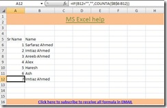
Take a look at image below which will guide you how to use this function on MS Excel worksheet.

Microsoft Excel and VBA help

The above code can be copied to module to use it. However, you are facing an issue with copying VBA code. Please download the file and to view code press Alt + F11 key.

Click here to download Extract Number example

Now, to use this code/VBA function in all Microsoft Excel file. You can download Add-ins which has this function embedded. There is another post on this blog to help you with installing Add-ins.

Click here to download Add-in

I would love to listen to you. Please write your comment below.

Subscribe here, its free.

We assure you knowledge, not SPAM!

Read more on this article...

Friday, August 7, 2009

VBA function to Concatenate

In this post, let's take a look at VBA code/function to concatenate string. Like in Microsoft Excel concatenate function you cant provide function with range. So you have to provide function with each cell at a time which is time consuming.  The best solution to help

VBA Code

Function VBAConcatenate(target As Range, delimiter As String) As String
Dim str As String

For Each c In target
    str = str + delimiter + c
Next c

If delimiter = "" Then
    VBAConcatenate = str
Else
    VBAConcatenate = Right(str, Len(str) - 1)
End If

End Function

VBAConcatenate require following parameters

Target: Target is range of cell you wish to concatenate.

Delimiter: Delimiter is any separator you want to use between concatenated text.

Example 1: You have A, B, C and D in range C6:C9 and you want the results as ABCD than you will use VBAConcate in following manner.

Formula: =VBAConcatenate(C6:C9,"")  will return ABC

Click on image below to view enlarge

Microsoft Excel, VBA concatenate

Example 2: You have A, B, C , D and E in range A6:E6 and you want the results as A|B|C|D|E  than you will use VBAConcate in following manner.

Formula: =VBAConcatenate(A6:E6,"|" )  will return A|B|C|D|E

Click on image below to view enlarge

Microsoft Excel, VBA Concatenate

Note this is very useful when you want to type a SQL query. In a query you need field name separated by comma. I use this function to get me list of field names in query.

You can also download the Microsoft Excel file with VBAconcatenate examples here. Just click on link below, to view code press Alt + F11

Click here to Download

The only issue with user define functions like VBAConcatenate is they remain limited to that MS Excel workbook where they are written. To use then in all workbooks on your system, you will have to convert this function into add-ins. So, once you install them on your computer you can use VBAConcatenate than in any workbook. You can download VBAConcatenate add-in here.

Click here to download Add-ins

If you need help with installing add-ins, please visit my earlier post How to install Add-ins.

Thanks for spending time in reading post. Request you to leave your comments. Also, you can receive updates, add-ins and e-books, its free.

We assure you knowledge, not SPAM!

Read more on this article...

Tuesday, August 4, 2009

Book Mark Add-in

Huge reports with more than 5 sheets are very difficult to browse. Also, in spite of making very professional report you will it confusing. So, solution to avoid confusion is to add book mark sheet with link to each Microsoft Excel worksheet. This worked in my case with large number of reports. But the process is very hectic. Like adding a shape, adding text to shape and than linking it to right worksheets which no one would like to do for each reports you make. Hence, I developed an MS Excel add-in which will automatically does these all for you. Take a look at the video below how it works.

How to use Bookmark Add-ins

This add-ins cost only 5$. If you like to receive this add-in click on button below to pay via Paypal. We will send you add-ins via email. Instructions to installation are available on my other post How to install add-ins.

If you want we will customize this add-ins to add your company name on Bookmark sheet, colors and font as per your need and customization will take only additional 5$.

Note: This add-ins is tested to work with MS Office 2003/2007. In case if you face any issue you can contact us and we will provide you support via email/chat.

Please suggest us your comments and feedback. Also, you can subscribe my blog. It’s free.

We assure you knowledge, not SPAM!

Read more on this article...

Wednesday, July 29, 2009

VBA Code to delete worksheets

In my last post we have seen how to add worksheets to Microsoft Excel workbook using VBA code. In this post we will delete the worksheet. Now, you have to be very careful while deleting worksheet because you won’t be able to recover any worksheet that deleted by using this VBA/Macro code. I have written two different set of codes. First one will delete active sheet while other one will delete based on sheet name provided by end user. I have purposely kept the prompt so that you don’t end up loosing any data while testing code.

So, let’s move ahead with first set of VBA/Macro code.

Sub DeleteActiveSheet()

' deletes active worksheet in the active workbook

On Error Resume Next

Dim str As String

str = ActiveSheet.Name

Sheets(str).Delete

End Sub

Warning: The above will permanently delete active worksheet. Kindly be careful.

Mentioned below is a second set of VBA/Macro code.

Sub DeleteSheet()

' deletes a sheet name entered by user in the active workbook

On Error Resume Next

Dim str As String

str = InputBox("Enter the worksheet name", "Findsarfaraz")

Sheets (str).Delete

End Sub

Warning: The above will permanently delete the worksheet name provide by you. Kindly be careful.

I would suggest you to take a look at code in MS Excel file. Click here to download. To view code, press Alt + F11 keys.

If you like to read more such articles, please subscribe to my blog. Click here to subscribe, its free. Also, your comments motivates me. Please comment.

We assure you knowledge, not SPAM!

Read more on this article...

Tuesday, July 28, 2009

VBA code to Add worksheet

Today we will discuss a different method in VBA to add worksheet in MS Excel workbook. Now when I say different method I mean ways of adding worksheet based on your requirement. Let’s moved ahead and start with simple piece of code to complex one in steps and based on scenario.

Scenario 1: Add worksheet with default name.

Sub Addsheet()

Worksheets.Add

End Sub

Note: The above code will add a worksheet before active worksheet.

Scenario 2: Add worksheet with specific name.

Sub Addsheet()

Worksheets.Add().Name = "Sarfaraz"

End Sub

Scenario 3: Add multiple worksheets.

Sub Addsheet3()

'Add Multiple worksheets

Worksheets.Add After:=Worksheets(Worksheets.Count), Count:=4

End Sub

Scenario 4: Add worksheets at end.

Sub Addsheet4()

'Add worksheets at the end

Worksheets.Add(After:=Worksheets(Worksheets.Count)).Name = "Sarfaraz"

End Sub

If you have any issue with replicating this code in MS Excel than download the Microsoft Excel file which I have uploaded. To view the code press Alt + F11 key on keyboard. To run the code I have place four buttons. Each button has one scenario.

Download Add Sheet example

For Free Microsoft Excel and VBA help subscribe to blog via email.

We assure you knowledge, not SPAM!

Read more on this article...

Monday, July 27, 2009

Sequence formula

Many a times you must want MS Excel to sequence the entry automatically. But thats not one of the features of MS Excel. So what you do is you enter the list than you type 1 in the top most row and drag it till last row. isn't it? This is most common practice I have seen around. Today here I will share to tricks on sequence.

In first sequence type, we will count the based on number of rows filled without checking if the value is duplicate with respect to previous row.

Formula: =IF(B6="","",COUNTA($B$6:B6))

In the above example, we are considering that we are sequencing based on column B starting from 6th row. The formula check if the value is present in B column and then counta find the count of non-blank from column B6 to respective row and returns count. Like, if you are on row 12 then formula will be  =IF(B12="","",COUNTA($B$6:B12)).  Lets take a look at illustration in image below.

Click on image below to view enlarge

Microsoft Excel, Sequence Generator

In second type, the increment happens only if the text entered is different from the one in the previous cell. Like if John is entered in B2 and B3 then both will have sequence number 1. Remember the same number will be assigned only if the both entered text are in adjacent cells like B2 and B3. Also, if you are using this for data entry purpose than to fix the sequence you can sort on the column.

Click on image below to view enlarge

Microsoft Excel, Sequence generator

Formula: =IF(B5="","",IF(B5=B4,A4,A4+1))

First IF checks whether the cells has any value. If the cells is empty then it leaves sequence cell empty(in above example A column has sequence numbers) empty. Else, it checks if the current cells values is same as cell in previous row. if yes, then it returns sequence of previous cell otherwise it adds 1 to sequence of previous row and return new number in sequence. You can concatenate/combine this sequence number with any text to get unique keys like in invoices/bill or memo.

I would suggest you to download the file I have enclosed with post. That will give you more clear picture. Also, I would suggest you to use this trick in one of your MS Excel report or template. So, you can remember entire logic.

Sequence example

Thank you for spending your valuable time in reading above post and if you like to read more such tricks subscribe to blog via email.

We assure you knowledge, not SPAM!

Read more on this article...

Friday, July 24, 2009

Trunc function to remove decimal

This function remove the decimal part of number. I find this function useful only when decimal precision is not important. Like you only want to consider 2 decimal places and want to completely ignore the numbers beyond 2 decimal places or so. The most important thing about Trunc function is it does not round off, it completely removes decimal.

Syntax: Trunc(Number, Precision)

We will take few number for example to explain you how Trunc functions works. Like in all other post, I have enclosed image with example.

Click on image below to view enlarge

Microsoft Excel, trunc

Also, if you face issue with replicating this example on MS Excel than download the MS Excel file with example.  I am sure you will use this function in your day to work life.

Download Example of Trunc

Thank you for spending your valuable time in reading above post and if you like to read more such tricks subscribe to blog via email.

We assure you knowledge, not SPAM!

Read more on this article...

Wednesday, July 22, 2009

Upper function to change case

This post is for beginners of MS Excel. This function convert all the characters to upper case(capitals). It is very useful when you have a data which is not in uniform case.  Like data received from Data entry operators.

Syntax: =Upper(Text)

Attached below is snapshot with Upper function as example. Take a look, I am sure this will help you.

Click on image below to view enlarge

Microsoft Excel, Upper Function 

There are other function in MS Excel which help you with cases are Lower(), Proper(). Also, the Upper function is very useful when you want to compare text from two cells. Since Exact() function is case sensitive it treats 'a' and 'A' as two different letters. I have enclosed the link to my earlier post where I have demonstrated to find cases using exact function

Check which CASE is used using Exact function

Thank you for spending your valuable time in reading above post and if you like to read more such tricks subscribe to blog via email.

We assure you knowledge, not SPAM!

Read more on this article...

Tuesday, July 21, 2009

Workday function

Workday function is used to find either past or future date before/after the given number of business days. The function only consider working/business days which mean while arriving to date it excludes Weekly off's and holidays. What I like most about this function is you can also provide it with holiday list you don;t want to be considered.

Now if you are thinking what will be the application of this function than let me tell you whenever I decide any dead line for project  I use this function to calculate date. This exclude all Weekends and holidays list which I provide to function. Also, this can be use to calculate delivery date or number of days of work performed.

Let's take a look at the syntax of formula below.

=Workday(StartDate, Days, Holidays)

StartDate is the beginning date

Days are the number of nonweekend and non-holidays days before or after start date which you want to use for calculating end date. Like for example, if you know that delivery of post takes 5 business days than you will input 5 to Days in formula.

Holidays: List of days you want to exclude while calculating end days. Like if you are not working on particular days than you can provide that to formula. This can be provided by using constant arrar {"A", "B","C"} or by range of cells. Remember, Saturday and Sunday are default weekends and will be considered as non working days.

Now lets take look at example of Workday function.

Click on image below view enlarge

workday function, microsoft Excel

To help you in making practical use of this formula I have made an MS Excel file with workday example and one of its application which you can download from link below. I foresee this function to be very useful when for companies who are in courier business. Also, in calculating targets for each employee and understanding time and motion calculation. Please do write to me if you like to discuss this further.

Click here to Download Workday function Example

Kindly do let us know your suggestion about post. Also, you receive free updates, add-ins, ebooks and useful macro code Click Here

We assure you knowledge, not SPAM!

Read more on this article...

Wednesday, July 15, 2009

VBA code, count using color

This is really funny thing in MS Excel I discovered today. Yes, a VBA code to count cells using colors. The intention behind is this post is to share VBA code and help you move ahead with VBA learning. This function is written by me. As you go below you will find formula syntax, vba code and add-ins. So, you can use add-ins on your system without replicating code and you can use this add-in all in open MS Excel file.

Syntax:  =CountColor(TargetRange,CellwithColor)

TargetRange: Range of cells which you wanted to count under which you want to count cells using criteria as another formatted cell.

CellwithColor: Single cell which filled with color which you want to count from TargetRange.

Note: It wont count cells that are formatted conditionally.

It may sound complex, but trust its very simple to use. Take a look at screen shot below where I have illustrated using CountColor.

Microsoft Excel, Count color 

Now, lets take a look a code of function which calculate count based on colors.

Public Function CountColor(target As Range, clr As Range) As Integer

Dim cnt As Integer

cnt = 0

For Each c In target
        If c.Interior.ColorIndex = clr.Interior.ColorIndex Then
            cnt = cnt + 1
        End If
Next c

CountColor = cnt

End Function

Dim cnt as Integer -> declare the integer variable used to count cells.

For each c in Target - > each c refers to one cell in target range while looping through for loop. So, if the target range is A1:A10 then while looping its goes A1, A2, A3.... ,A10.

c.Interior.colorIndex -> Colorindex returns the number for color, Interior of cell refers to color pattern and c is cell from target range. Similarly, clr.Interior.ColorIndex returns the number for color pattern in criteria.  So, if the number returned by getcolorindex method matches with number returned by getcolorindex of criteria it adds 1 to cnt.

After completing the entire range it pass the value to Countcolor.

If you still have doubts, download the count color example file. I am sure you would love to use this function.

Download Count color example

Macro are good to use when you want to process or perform operation in one MS Excel file. However, when you want to use any function/vba code independently in all open MS Excel file than add-ins are the best option. Other good thing about add-ins is they don't prompt whether you want to enable or disable code. Hence, I have uploaded the add-ins for you to use and send it across to your friends. Please feel free to download, its Free.

 Download Countcolor Add-ins

If you need help with installing add-ins, please visit our post How to install Add-ins.

Thanks for spending time in reading post. Request you to leave your comments. Also, you can receive updates, add-ins and e-books, its free.

We assure you knowledge, not SPAM!

Read more on this article...

Tuesday, July 7, 2009

Year Function

Year function is used to extract year from Date. It’s very useful when you want to summarize data at year level or you want to apply filter on year. This function in combination with other function is very useful in calculating past/future dates. I will share few examples of Year function in near future.

Formula: =Year(Date)

Click on image below to view enlarge

Yearfunc

Example1: Find the current year.

Formula: Year(Today())

Click on image below to view enlarge.

yearfuncexam

If you face any issue with replicating this example in MS Excel or understanding this function. I would suggest you to download Year function Excel file enclosed below

Year Function Example

Kindly let me know your view and experiences about using Year function. For free updates subscribe here.

We assure you knowledge, not SPAM!

Read more on this article...

YearFrac Function

Yearfrac functions returns the portion of years between dates. The most recommended format of return is percentage. Like if you take Jan 01, 2009 as start and Jun 30, 2009 as end, YearFrac will return 0.49 which is nothing but 49% of year. 

 Formula: Year(StartDate, EndDate, Basis)

StartDate: StartDate is date as the name suggest is beginning date which you want to be considered for calculation. Like, if you want to calculate fraction of year starting from day one of year than start date will be 01/01/2009.

EndDate: Similar as above will be last date till which you want to find the fraction of year.

Basis: There are five options available for choose based on which you will receive the results. Each Type is mentioned below.

  • 0: US Calendar style where 30 days per month is considered and hence 360 days in a year. Like 30/360. Also, if nothing is provided in basis than by default if consider as 0.
  • 1: This will make formula take actual number of days/actual number of days year consist of.
  • 2: Actual number of days/360.
  • 3: Actual number of days/365.
  • 4: Eurpean 30/360

Basis is a most critical parameter which will be be dependant of type of calendar you follow or you want to use for calculation. So, be sure.

Example 1: We will try to calculate YearFrac using different basis.  Just to keep the example started I will considered fixed dates 7/6/2009 and 8/6/2009 which has different of 31 days between them.

Click on image to view enlarge.

yearfrac

Example 2: Task is to calculate leaves on pro-data basis. Like in a year you can have only 21 leaves. So, as the days passes how many leaves will accumulate.

Click on image to view enlarge.

YearFrac2

Note: in both examples I have formatted Yeafrac as percentage.

If you still have difficulty in using YearFrac function. I would suggest you to download the file with YearFrac Example. Also, I have added on bonus example in this file.

Click Here to download YearFrac

If you are first time visitor I would request you to subscribe our blog via Email. We will send you free tutorials, e-books, Add-ins and macro code.

We assure you knowledge, not SPAM!

Read more on this article...

Monday, July 6, 2009

Format Painter

Format painter is very useful tool when you only wanted to move format of one cell to another or range on worksheet. Using format painter is easiest way to replicate format on the worksheet.

format painter icon  is a format painter icon which you will find on Standard toolbar.

Follow the steps to use format painter to move format.

  1. Select the cell of which you want to copy the format.
  2. Click on the format painter icon icon on Standard toolbar.
  3. The moment you click on Format painter icon, you will see that your cursor has changed to + paintbrush icon.
  4. Now you can apply the format by clicking on single cell or by dragging it on range of cell. However, if you want to apply the format to disjoint/non contiguous cells than steps will be bit different.

Follow the steps to use format painter on non-contiguous cells.

  1. Select the cell of which you want to copy the format.
  2. Double click on the format painter iconformat painter icon on standard toolbar.
  3. Now, like earlier the moment you double click the format painter icon you will see your cursor has change to + paintbrush icon.
  4. Now, click on all the cells of which you want to change the format. Once you are done, press Esc.

During my first few month's as an MIS I used this method to speed up my work. Format painter very well copy the conditional formatting as well which I liked the most. Remember one thing, more you practice, more you learn. So, keep practicing. I have one more idea of moving format which I will share with in future posts. Do miss any post, its Free!.

We assure you knowledge, not SPAM!

Read more on this article...

Wednesday, July 1, 2009

Countif with wildcard criteria

Here we will learn to use wildcard * in Countif function. Task is find count of all cell which starts with A or any character. There may be many ways which I may not be aware of, here I am posting something I tried and it worked. If you are not comfortable with Countif than this post is not for you. I would suggest you to visit my Countif Function.

Syntax for countif function is as follows : Countif(Range, Criteria)

Example: We wanted to find count of names starting with A and Sa from the list of names in A column of sheet. Suppose the names are in A2 to A10 range.

Formula Countif(A1:A10, "A*") will return the count of all names starting with A and Countif(A1:A10, "Sa*")

Click on image to view enlarge.

Microsoft Excel, countif example

Note: Criteria provided in countif is not case sensitive. SA and Sa will be treated as same.

Also, you can use this function with conditional formatting for give specific color to cell starting specific character.

You can also download an Countif with wild card example file. 

Click here to download Countif Example

If you are first time visitor, please subscribe via email to receive updates, add-ins, e-books and lot more.

We assure you knowledge, not SPAM!

Read more on this article...

Friday, June 26, 2009

Add-in and macro to convert seconds to hh:mm:ss

This add-in and macro will help you in converting seconds to hh:mm:ss. I have put add-ins for those who just wants to use the add-ins and macro for those who wants to understand this trick. This is very useful in BPO/Contact Center where you have source data in seconds and you have to represents data in hh:mm:ss seconds.

Mentioned below is macro code

Sub convert_hh_mms_ss()
Dim i As Double
Dim x As Integer
Dim y As Long
x = 1
y = 1
For Each c In Selection
    i = c / 86400
    Selection.Cells(x, y) = i
    Selection.Cells(x, y).NumberFormat = "[h]:mm:ss;@"
    x = x + 1
Next c
End Sub

Logic: c is each cell in selection/range on which you want to perform conversion. 86400 is nothing but the number of seconds in a day ( 24*60*60). When you divide seconds(c/86400) with 86400 it returns the numeric value in which MS Excel stores the time. In next steps we convert this numeric value into time format.

If you have difficulty replicating the code in MS Excel. Please download the example file.

Download Macro Example

Also, if you can use this macro as Add-in. Dow

Download Add-ins

If you need help with installation of Add-ins, please follow our earlier post

How to install Add-ins

Please do let me know your comments about this macro and add-ins. Also, you can subscribe via email to receive latest updates, add-ins and e-books in your inbox.

We assure you knowledge, not SPAM!

Read more on this article...

Tuesday, June 23, 2009

Remove password

Few days back I wish to remove the password from protected file. So, I started hunting for password removers for MS Excel in Google. I found a unique utility to quickly remove the password which I wanted to share with you all. The reason I am posting this here is there are many such utility available and few of them are paid as well. Also, I have already tested it by putting strong passwords.

Download Password remover Add-in

This utility is in the form of Add-in. So, click on the link below to follow the installation instruction.

How to install MS Excel add-ins

I would like to convey the special thanks to the developer. Kindly visit them as well

http://www.straxx.com/excel/password.html

Kindly let us know your comments about your experience about using this add-ins. To receive more such add-ins, e-books and MS Excel updates subscribe to us via email

Disclaimer: This add-ins is not developed by me, nor I am anyway associated to the developer. To view developer site click here

We assure you knowledge, not SPAM!

Read more on this article...

Monday, June 22, 2009

VBA to close excel.exe

Closing all orphan Excel.exe process

I came across this issue while I was generating reports on SQL server using MS Excel. Here we use to generate reports using MS Excel macro. However this macro's where executed via DTS in SQL. At times if any error occurs, the DTS use to close down leaving excel.exe running as orphan object. This not only sometimes prevent other excel objects but also slow downs your server performance. To tackle this we used the following code to close all MS Excel objects before opening new object.

Sub Close_Excel()

Dim strClsExl As String
strClsExl = "TASKKILL /F /IM Excel.exe"
Shell strClsExl, vbHide

End Sub

Warning: Kindly save all your work before trying above code as this will close all MS Excel instances running on computer and you will end up loosing your work.

For your convenience I have linked two files for download along with this post. One has Macro example which you can in understanding code while other is an add-in which will can directly install in your MS Excel. Also, in add-in I have let user to decide which .exe file they want to close.

Download Close Excel example

Add-ins to close exe

If you need more help with installing add-in on your computer do visit our other post which is mentioned below.

Install Add-ins help

Kindly leave your comments about this post and receive more such add-ins by subscribing us.

We assure you knowledge, not SPAM!

Read more on this article...

Monday, June 15, 2009

Weekday function

This function is used to find day of week from Date. Also, you can decide which day of week you want to begin the week. Like for different organizations have different week beginning and ending. We will first understand syntax  and than move on two unique use of Weekday function.

Syntax: = Weekday(DateEntered, WeekStart)

WeekStart =1 sets Sunday as start that is 1  and Saturday as end which will7

WeekStart = 2 sets Monday as start that is 1  and Sunday as end which will be 7

WeekStart = 3 sets Tuesday as start that is 1 and Monday as end

If you don't provide any WeekStart then by default MS Excel assume it to 1.

Take a look at image below with weekday formula. 

Click on image below to view enlarge

Weekday function, MS Excel

Example 1: We want to find out day name using weekday function.

Note: The cell format should be choosen as dddd in custom formatting. To choose cell formatting, Press Ctrl + 1 and select custom from category and type dddd.

Example 2: Format entire rows where day is Monday. This is very useful when your week start/end at Monday and you want to mark start or end of week.

Click on image below to view enlarge

 weekexmple2

Here the entire row is formatted based of the value present in A column. If you still have confusion, download the file with Weekend function.

Download Weekday function Example

Also, do let me know your comments about this post and subscribe to us to receive latest updates via email

We assure you knowledge, not SPAM!

Read more on this article...

Saturday, May 16, 2009

INT function

INT rounds of the number to lowest and nearest whole number. INT function does not require any special formatting.

Syntax: INT(Number)

Number Integer Formula
3.5 3 =INT(3.5)
7.2 7 =INT(7.2)
15.99 15 =INT(15.99)
-22.7925 -23 =INT(-22.7925)

Example: A competitive exams require the 18 years of age to appear in exams.  Here is example on finding candidate with age over 18.

Click on image to view enlarge

INTFUNCTION

I have uploaded the MS Excel file with INT function and INT function example to ensure that we don't miss anything with respect to basic understanding of INT function.

Also, do let me know your comments about this post and subscribe to us to receive latest updates via email

INT function Example

We assure you knowledge, not SPAM!

Read more on this article...

Friday, May 15, 2009

Rand and Randbetween function to generate random numbers

Rand and Randbetween is used to generate random numbers. It is very useful for people like me who post on blog. This help me in generating random data which I use in post on blog. Randbetween is available in MS Excel 2007 while RAND function is available in MS Excel 2007/2003/XP/2000. Randbetween function has an edge over Rand function as it can generate numbers between lower bound and upper bound and gives user a control to over generation of random numbers.

Rand() Function

Syntax: Rand()

RAND() function does not require any special formatting. However it returns number in decimal or in others words it returns you number between 0 to 1. Take a look at the image below with example of RAND() function.

Click on image  to view enlarge

rand

Randbetween() function

Syntax: RANDBETWEEN(LOWER, UPPER)  is syntax for RANDBETWEEN() function in MS Excel 2007.

Like Rand() function, Randbetween() function does not require any special formatting. Take a look at image below to view example of Randbetween() function.

Click on image  to view enlarge

randbetween

 Example: The example exhibits how to use RAND() function to generate numbers between fix range.

Click on image  to view enlarge

rand_example

Mentioned below is RAND() function along with INT function and is equivalent to RANDBETWEEN function of Excel 2007. 

Formula: INT(RAND()*(b-a)+a)

here a= 100 and b=200

=INT(RAND()*(200-100)+100)

(200-100) returns 100 which when multiplied with RAND() return two digit number. Also, here it is treated as upper bound and lower bond. In other words, this function will return numbers between 100 and 200. You can try with different numbers.

RAND()*(200-100)+100 adds to 3 digit number which is greater than 100 but less than 200. Also, some decimal.

INT functions round off to lowest integral value.

If you are still in doubt using RAND() and RANDBETWEEN() function. I have kept the file with example for download

Random Number Example download

To receive more updates on MS Excel help. You can subsribe via email.

We assure you knowledge, not SPAM!

Read more on this article...

Wednesday, May 13, 2009

Product function

This is simple multiplication function. Very useful in almost all worksheet. However, we prefer to use other alternative to multiply numbers. The alternative to Production function is using cell reference in following manner:  A1*B1*C1 which is equivalent to Product(A1,B1,C1)

Syntax

=Product(number1, number2, number3........,number30)

=Product(Rangeofnumbers)

=Product(number, Rangeofnumbers)

Click on image below

Product

You can download the file with Product formula example. I am sure this will help you in learning this function.

Download Product Example File

Please do let me know your comments about my attempt to help beginners with Product function. Also, you can subscribe via email

We assure you knowledge, not SPAM!

Read more on this article...

Monday, May 11, 2009

Shortcut key to enter Date and Time in worksheet

Using NOW function refreshes each time when you make entry to worksheet. Hence, I dont prefer to use NOW function. I use shortcut key to enter time or Date to worksheet.  This trick is helpful in saving time.

For Time

Shortcut key: Ctrl + Shift + ;

For Date

Shortcut key: Ctrl + ;

Please do let me know your comments about my attempt to help beginners with Shortcut key to enter date and time. Also, you can subscribe via email

We assure you knowledge, not SPAM!

Read more on this article...

Now function for Time

Now function is used to enter current date and  time. The Now function keeps on updating time whenever you open workbook or when you make entry to worksheet. This function is useful when you want to use current date and time.

Formula: Now()

Now function returns date and time. However the format of cells plays very important role. Click on the image below to take a look of different cells formatted returns date and time in different date and time formats. In simple words, Now functions returns date and time based on cell format.

Click on image to view enlarge

nowfunction

For further help, you may download MS Excel file with Now function example.

Now Function Example download

Please do let me know your comments about my attempt to help beginners with Now function. Also, you can subscribe via email

We assure you knowledge, not SPAM!

Read more on this article...

Saturday, May 2, 2009

SUMPRODUCT function

The SUMPRODUCT in MS Excel is useful when you want a multiple a set of values to another set of value. This formula is very useful in scenario when you want to calculate the total sales value or cost. Let's take look at syntax.

Syntax: SUMPRODUCT(array1, array2, array3....)

Table

Set A Set B
a1 b1
a2 b2
a3 b3
a4 b4
. .
an bn

SUMPRODUCT({a1, a2, a3, a4...an}, {b1, b2, b3, b4...bn}) = a1 X b1+a2 X b2+a3 X b3+a4 X b4....an X bn

Click on image below to Enlarge


In the above example, we have describe an example to calculate Total sales value and Total Cost value. Also, I have enclosed the link with example of SUMPRODUCT formula.

Click here to download SUM Product Example

Kindly let me us know your comment about this post. Also, you can subscribe to this blog to receive latest update in your inbox. Click on the link below

Subscribe to blog via Email

We assure you knowledge, not SPAM!

Read more on this article...

Thursday, April 30, 2009

VBA, For Next loop

For next is looping method when you are definite about number of values you want to scan/test. However, you will have to use IF then to test the values. Lets take a look at very basic example of For Next loop and then we will move at little complex examples.

Syntax:

For counter = startvalue to endvalue
    Operation you want to perform
Next counter
Next counter increase the value to loop till counter reaches end value

Here you want to just enter random numbers starting from active cell to next 10 row using VBA/Macro code

For Next loop Example 1

Sub Fornextloop1()
Dim i As Integer

'We will use i as counter
For i = 0 To 9
    ActiveCell.Offset(i, 0) = WorksheetFunction.RandBetween(25, 250)
Next i

End Sub

Note: Code     ActiveCell.Offset(i, 0) = WorksheetFunction.RandBetween(25, 250) may not work with MS Office 2003 or previous version. Please replace the following code with

ActiveCell.Offset(i, 0) = WorksheetFunction.Rand(25, 250)

Similary, if you want to list of 10 values of actual and 10 values of target lying in set of adjacent cells and you want to find out whether actual have exceeded the target or not.

For Next loop Example 2

Sub Fornextloop2()
Dim i As Integer
'We will use i as counter
For i = 0 To 9
    If ActiveCell.Offset(i, 0) >= ActiveCell.Offset(i, 1) Then
        ActiveCell.Offset(i, 2) = "MET"
    Else
        ActiveCell.Offset(i, 2) = "NOT MET"
    End If
Next i

End Sub

Here in the above examples we are taking increment of 1 only. In case if you want to have increment of more than 1 than you can take look at example where I have illustrated Example 1 but you only want to put even numbers. Like 2, 4, 6.... 20

For Next loop Example 3

Sub Fornextloop3()
Dim i As Integer

'We will use i as counter
For i = 0 To 20 Step 2
    ActiveCell.Offset(i / 2, 0) = i
Next i
End Sub

Step 2 makes the counter incremented by 2 each time. Also, i / 2 under offset ensures that each value in inserted in row. Only i will insert values in alternate cells.

You may think is it necessary always to increase value of counter can't we decrease the value of counter. Yes, we can do that as well. Next example illustrate the same. Now, we want to scan all the rows starting from 40th row and move to 1st row. Also, we want to highlight values above certain threshold (Here I have take 30 as threshold).

For Next loop Example 4

Sub Fornextloop4()
Dim i As Integer
'We will use i as counter
ActiveSheet.Cells(1, 1).Select
For i = 39 To 1 Step -1
     If ActiveCell.Offset(i, 0) > 30 Then
        ActiveCell.Offset(i, 0).Interior.ColorIndex = 3
    End If
Next i
End Sub

Step -1 decreases the value of i by 1.

Next example will shows us how to run nested For Next loop which is of extremely use full when you want to move across rows and columns at a time. I am using the example similar as previous one.

For Next loop Example 5

Sub Fornextloop5()
Dim i As Integer
Dim j As Integer
'We will use i as counter
ActiveSheet.Cells(1, 1).Select
For i = 11 To 1 Step -1
    For j = 11 To 1 Step -1
        If ActiveCell.Offset(i, j) > 30 Then
            ActiveCell.Offset(i, j).Interior.ColorIndex = 3
        End If
    Next j
Next i
End Sub

I am sure this post will help you in applying For Next Loop. In case if you find difficult to use in your MS Excel Sheet. I would suggest you download file with Example. Press Alt + F11 to view code and press Alt+ F8 to run the code.

For Next Example

Please do let me know your comments about my attempt to help beginners with For Next loop. Also, you can subscribe via email

We assure you knowledge, not SPAM!

Read more on this article...

Wednesday, April 29, 2009

VBA, Do while Loop, Do loop until

This is every useful VBA loop as it can be used for indefinite range with conditions applied. Like when you wanted to test starting to row 1 to last non-empty row or want to run macro for any particular condition only. You should remember that there is counter used for increment and this counter has to be part of criteria and there is Loop statement which rounds off the Do while statement. Loop is similar to Endif in IF Then or Next statement in For next loop as we have seen in my previous posts.

Syntax:

Do While (Criteria)
    counter = counter + 1
    'counter is has to be part of criteria
Loop

Do     counter = counter + 1
    'counter is has to be part of criteria
Loop While/Until (Criteria)

Now, lets look at few examples on Do loops. I am sure these examples will help you in learning if you practice them.  Incase if you face any issue with replicating this code, please download the example file which has all example to try hands on. Also, you can make changes in code to test and enhance your skills.

Example 1:  Sheet named 'Dowhile_DoUntil1' has data of all the cities with their scores. We want to scroll till non-empty row and want to display number of non-empty row.  Remember we are only testing column 1.

-------------------------------------------------------------------------------------------------------------------------------

Sub Dowhile1()

Dim i As Long

'i is initialize to one as 1 is the minimum row on excel sheet and is very important step

i = 1

Do While Sheet1.Cells(i, 1) <> ""

i = i + 1
Loop
MsgBox "Last non-empty row is " & i - 1

End Sub

-------------------------------------------------------------------------------------------------------------------------------
Sub Dountil1()

Dim i As Long

i = 1

'i is initialize to one as 1 is the minimum row on excel sheet and is very 'important step                                                                                                                
Do
    i = i + 1
Loop Until Sheet1.Cells(i, 1) = ""

MsgBox "Last non-empty row is " & i - 1

End Sub

-------------------------------------------------------------------------------------------------------------------------------

If you observe carefully you will find the condition in Do while (While Sheet1.Cells(i, 1) <> "" )and Do Until (Until Sheet1.Cells(i, 1) = "")  is exactly opposite.

Example 2: We want to move and test across rows and columns., Like matrix. For all cells containing more than 150 should be colored green and below 50 should be marked red. In practical use I would even prefer to use conditional formatting if I have to only use two formats. But actually you can use for this for having n number of conditional formats.

-------------------------------------------------------------------------------------------------------------------------------

Sub Dowhile2()

Dim i As Long
Dim j As Integer
i = 1
j = 1

Do While Sheet2.Cells(i, j) <> ""

    Do While Sheet2.Cells(i, j).Value <> ""
        If Sheet2.Cells(i, j) < 50 And IsNumeric(Sheet2.Cells(i, j)) = True Then
            Sheet2.Cells(i, j).Interior.Color = vbRed
        ElseIf Sheet2.Cells(i, j).Value > 150 And IsNumeric(Sheet2.Cells(i, j)) = True Then
            Sheet2.Cells(i, j).Interior.Color = vbGreen
        ElseIf (Sheet2.Cells(i, j).Value >= 50 And Sheet2.Cells(i, j).Value <= 150) And IsNumeric(Sheet2.Cells(i, j)) = True Then
            Sheet2.Cells(i, j).Interior.Color = vbYellow
        End If
    i = i + 1
    Loop
j = j + 1
i = 1
Loop

End Sub

-------------------------------------------------------------------------------------------------------------------------------

Sub Dountil2()

Dim i As Long
Dim j As Integer
i = 1
j = 1

Do

    Do
        If Sheet2.Cells(i, j) < 50 And IsNumeric(Sheet2.Cells(i, j)) = True Then
            Sheet2.Cells(i, j).Interior.Color = vbRed
        ElseIf Sheet2.Cells(i, j).Value > 150 And IsNumeric(Sheet2.Cells(i, j)) = True Then
            Sheet2.Cells(i, j).Interior.Color = vbGreen
        ElseIf (Sheet2.Cells(i, j).Value >= 50 And Sheet2.Cells(i, j).Value <= 150) And IsNumeric(Sheet2.Cells(i, j)) = True Then
            Sheet2.Cells(i, j).Interior.Color = vbYellow
        End If
    i = i + 1
    Loop Until Sheet2.Cells(i, j).Value = ""
j = j + 1
i = 1
Loop Until Sheet2.Cells(i, j) = ""
End Sub

-------------------------------------------------------------------------------------------------------------------------------

IsNumeric(Sheet2.Cells(i, j)) = True test whether the value is numeric or not. IsNumeric() is very useful while scanning range of cells and you want to check or apply code only to cell with numeric values.

I will post some tips where you will see an extensive use of Do while/Until loop in MS Excel/VBA as Do while/until is most useful loop. Also, for your convenience I have posted link to download MS Excel file.

Download Do while/Until Loop

Kindly let us know your comments about this post.

Subscribe to blog via Email

We assure knowledge. Not SPAM.

Read more on this article...

Tuesday, March 31, 2009

VBA, IF then condition

IF THEN: IF Then is use to perform comparison two values. However, to perform the test for set of data you will have to use IF then with Do while or For Next loop.

Lets take a look at basic IF Then example with single condition.

Sub LoopIFThen1()
If ActiveCell.Value >= 18 Then
    MsgBox "You are Major"
Else
    MsgBox "You are Minor"
End If
End Sub

If the active cell has value more than or equal to 18 then message box will appear saying "you are 18" otherwise nothing will happen.

Now, we will use IF then to see alternate condition as well. Alternate condition is like what should code perform if active cell is less than 18.

Sub LoopIFThen2()
If ActiveCell.Value >= 18 Then
    MsgBox "You are Major"
Else
    MsgBox "You are Minor"
End If
End Sub

After trying to simple example we will move little complex example with multiple condition. Like if the active cell has age entered than in next cell it will tell you whether you are infant, minor, major or senior citizen.

Sub LoopIFThen3()
If ActiveCell.Value < 2 And ActiveCell.Value <> "" Then
    ActiveCell.Offset(0, 1) = "Infant"
ElseIf ActiveCell.Value > 2 And ActiveCell.Value < 18 And ActiveCell.Value <> "" Then
    ActiveCell.Offset(0, 1) = "Minor"
ElseIf ActiveCell.Value >= 18 And ActiveCell.Value <= 60 And ActiveCell.Value <> "" Then
    ActiveCell.Offset(0, 1) = "Major"
ElseIf ActiveCell.Value > 60 And ActiveCell.Value <= 100 And ActiveCell.Value <> "" Then
    ActiveCell.Offset(0, 1) = "SENIOR CITIZEN"
Else
    MsgBox "Please check Value"
End If
End Sub

In Above example, Activecell(0,1) refers to next column in right. In forthcoming post, we will use other loops like Do while, For Next loop along with IF Then. Also, you if you have problem trying this example then try downloading the file with example. Link for same is mentioned below

Download IF Then Example

Please post your comments about the post and subscribe via email to receive latest updates

We assure you knowledge, not SPAM!

Read more on this article...

Monday, March 23, 2009

Shortcut to show all formula

At times I have seen people validating data and formula's on MS Excel sheet. It's very tedious if you go to each cell to view formula. Here is short cut to reveal all formulas. Trust me its very useful while auditing data in MS Excel

Shortcut key: Ctrl + `

Now if you have difficulty locating ` key. Let me help you, on most of standard keyboard `is located before 1 key or above tab key.

In last few months, I have posted lot of MS Excel Basic posts to ensure that everyone has something to learn who spare time and visit my blog.  As an advice I will say that learn one shortcut/formula in a day. Very soon you will be many other who do not follow this practice.

I would appreciate if you provide comments and subscribe via email to get latest email.

We assure you knowledge, not SPAM!

Read more on this article...

Wednesday, March 18, 2009

Countif function

This function works like SUMIF function. Like in last post I am using the same example. As the name suggest, COUNTIF finds the count based on criteria provided by user. Very useful when you are summarizing data or excluding unwanted  by setting criteria. Also, in forthcoming post I will provide examples of COUNTIF function that too in complex formula's. I will summarize data from baby product sales using Countif. 

Formula: =COUNTIF(RangeOfThingsToBeCounted ,CriteriaToBeMatched)

Here is example below which show day-wise baby product sales.

Date Item Quantity Cost Amount
17-Mar-09 Dolls 44 148 6512
12-Jan-09 Hairpin 8 57 456
15-Apr-08 Diapers 8 176 1408
28-Jun-08 Baby Oil 29 124 3596
24-Nov-09 Dolls 43 120 5160
16-Oct-09 Diapers 34 159 5406
24-Mar-09 Baby Oil 39 196 7644
16-Jan-09 Diapers 26 154 4004
17-Apr-08 Dolls 28 84 2352
4-Jul-08 Baby Oil 39 82 3198
28-Nov-09 Diapers 36 101 3636
20-Oct-09 Cap 30 117 3510
3-Apr-09 Dolls 17 122 2074
23-Jan-09 Cap 45 55 2475
25-Apr-08 Dolls 6 93 558
        51989

The task here is to find count of each product in summary table based on Item name. So item name is criteria here. 

Table below shows part one where we want to summarize the sales table item-wise.

Range part of COUNTIF covers B2:B16 examines which cells has item name, B22 has Doll which it takes as Criteria can only count where it finds respective items.

Items Count Formula
Dolls

5

=COUNTIF(B2:B16,B22)
Hairpin

1

=COUNTIF(B3:B17,B23)
Diapers

4

=COUNTIF(B4:B18,B24)
Baby Oil

3

=COUNTIF(B5:B19,B25)
Cap

2

=COUNTIF(B6:B20,B26)

Another examples below demonstrates find count of items where count if greater than 25.

Criteria Total Formula
Count where Quatity >25

11

=COUNTIF(C2:C16,">25")

Range part of COUNIF covers C2:C16 examines quantity column which cells has number greater than 25. Here Criteria is a string ">25".

I am sure this post is helpful in understanding COUNTIF function. Post your comments

I am sure after SUMIF in the last post, you will find COUNTIF easy. Enclosed is link to download the COUNTIF Example

COUNTIF Example download

If you are first time visitor, please subscribe via email to receive updates, add-ins, e-books and lot more.

We assure you knowledge, not SPAM!

Read more on this article...